Suppose you are an HR professional and want to determine:
- Whether age of an employee has a substantial effect on their maturity
- The importance of experience and capability on remuneration
- The importance of IQ (Intelligence Quotient) vs. EQ (Emotional Quotient) on problem handling capability
- How sedentary lifestyle at workplace affects employee output
- If a specific physical activity makes employees more energetic and lively at the workplace
All these are routine scenarios in an organization. But their impact is huge. How, as an HR professional, can you determine which variables have what impact on employee productivity?
Regression analysis offers you the answer. It helps you explain the relationship between two or more variables.
With Explanation Comes Consideration!
However, before we go into details and understand how regression models can be employed to derive a cause and effect relationship, there are several important considerations to take into account:
- Not all assumptions can be tested and validated.
- You need to carefully establish a hypothesis, for it to work out correctly.
- Accuracy of results depends upon authenticity of data.
- Ignoring important variables can bias your coefficients.
- The econometric model you choose should fit the type of data you’re using.
Linear Regression Model
Regression analysis simplifies some very complex situations, almost magically. It helps researchers and professionals correlate intertwined variables. Linear regression is one of the simplest and most commonly used regression models. It predicts the cause and effect relationship between two variables.
The model uses Ordinary Least Squares (OLS) method, which determines the value of unknown parameters in a linear regression equation. Its goal is to minimize the difference between observed responses and the ones predicted using linear regression model. There are certain requirements that you need to fulfill, in order to use this model. Otherwise the results can be confusing and ambiguous.
Prerequisites of using a linear regression model
- The number of observations is finite.
- The primary assumption is that there are negligible errors in the value of independent variable (X) or regressor variables. It follows the principle of strict exogeneity, which means zero error.
- Regressors or independent variables should be predefined constants or random variables.
- Smaller the differences between data point corresponding to the regression line, better an econometric model fits the data.
- It provides the maximum likelihood estimator, maximizing the agreement of the selected econometric model with the observed data.
Let’s understand it with the help of an example:
The phenomenon is: Work experience and remuneration are related variables. The linear regression model can help predict the remuneration slab of an employee given his/her work experience.
Statistical Representation
Now the problem arises how to represent it statistically.
There are two lines of regression – Y on X and X on Y.
Y on X is when the value of Y is unknown. X on Y is when the value of X is unknown.
Here are their statistical representations:
Suppose, the value of remuneration is = Y and the value of experience is = X
| The Line of Regression of Y on X | The Line of Regression of X on Y | Then, to predict the unknown value of remuneration (Y), the statistical representation will be: | If it is the other way around or the value of work experience is unknown, the statistical representation will be: | Y = a + b(X) | X = c + d(Y) | Where ‘b’ is the coefficient of X and ‘a’ is the intercept of Y. | Where ‘d’ is the coefficient of Y and ‘c’ is the intercept of X. |
|
Selection of Line of Regression
The statistical representation above is an example to show how to develop econometric models when the value of one of the variables is known and another’s unknown. However, this doesn’t mean that both the representations are correct.
This is because remuneration may depend on the work experience of an individual but the vice versa is not true. Experience doesn’t depend on remuneration. Therefore, you’ll have to carefully choose the dependent variable and then the line of regression.
What Does a Regression Equation Mean?
A linear regression equation shows the percentage increase or decrease in the value of dependent variable (Y) with the percentage increase or decrease in the value of independent variable (X).
Let us suppose the values of X and Y are known.
Table 1
Graphically it’s represented as:
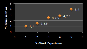 Graph 1
The white line connecting all the dots in the graph above represents the error or prediction. But you now want to find the best-fitted line of regression to minimize the error of prediction. The aim is to help find the best-fitted line of regression.
How to Find the Best-Fitted Line of Regression?
By using the ordinary least squares method!
Let us continue with the above example:
Table 2
| | X | Y | XY | X-X’ | Y-Y’ | (X-X’)(Y-Y’) | (X-X’)2 | (Y-Y’)2 |
| | 1 | 1 | 1 | -2 | -1.16 | 2.32 | 4 | 1.346 |
| | 2 | 1.5 | 3 | -1 | -0.66 | 0.66 | 1 | 0.436 |
| | 3 | 2.5 | 7.5 | 0 | 0.34 | 0.34 | 0 | 0.116 |
| | 4 | 2.8 | 11.2 | 1 | 0.64 | 0.64 | 1 | 0.410 |
| | 5 | 4 | 20 | 2 | 1.84 | 3.68 | 4 | 3.386 |
| Sum | 15 | 10.8 | 42.7 | | | 7.64 | 10 | 5.69 |
| Mean | X’ = 3 (15/5) | Y’ = 2.16 (10.8/5) | | | | | | |
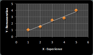 Graph 2
The primary equation is:
Y = a + b(X) +e (error term)
In this case, e is zero because it is assumed that the independent variable (X) has negligible errors.
Therefore, it remains Y = a + b(X).
Let us now find the value of b.
b = [ ∑ XY – (∑Y)(∑X)/n ] / ∑(X-X’)2
Substitute the values in the above formula:
b = [ 42.7 – (15*10.8)/5 ]/10 = [ 42.7 – 162/5 ]/10 = [ 42.7 – 32.5 ]/10 = 10.2/10 = 1.02
b = 1.02
Therefore,
a = Y – b(X)
a = Y – 1.02(X) or a = ∑Y/n – 1.02 (∑X/n)
a = 2.16 – 1.02*3 = 2.16 – 3.06
a = -1.06
By substituting the value of a, b and X, we can find the corresponding value of Y.
Y = a + b(X) = -1.06 + 1.02X
When X = 1
Y = -1.06 + 1.02*1 = -0.04
When X = 2
Y = - 1.06 + 1.02*2 = 0.98
When X = 3, Y will be 2
When X = 4, Y will be 3.02
When X = 5, Y will be 4.04
Table 3
| X | Y |
| 1 | -0.04 |
| 2 | 0.98 |
| 3 | 2 |
| 4 | 3.02 |
| 5 | 4.04 |
The best-fitted regression line will be:
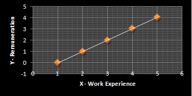 Graph 3
Properties of the Best-Fitted Regression Line/Estimators
- The regression line passes through the X’, which is 3 in this case. (Refer to Graph 3)
- b, the regression coefficient of X, is an average change in Y. In this case, b = 1.02 which is the average change in the values of y: -0.04, 0.98, 2, 3.02 and 4.04. (Refer Table 3)
- The regression line passes through Y’, which is 2.16 in this case. (Refer Graph 3)
Coefficient of Determination – Assessing Goodness-of-Fit
Whenever you use a regression model, the first thing you should consider is – how well an econometric model fits the data or how well a regression equation fits the data.
This is where the concept of coefficient of determination comes in. The regression models are generally fitted using this approach.
It determines the extent to which dependent variable can be predicted from independent variable. It assesses the goodness-of-fit of the Ordinary Least Square Regression Model.
Denoted by R2, its value lies between 0 and 1. When:
- R2 = 0: the value of the dependent variable cannot be predicted from the independent variable.
- R2 = 1, the value of dependent variable can be easily predicted from the independent variable. There are no errors in the data.
Higher the value of R2, better fit the model is to the data.
Let’s now understand how to calculate R2. The formula for finding R2 is:
R2 = { (1 / n) * ∑ (X-X’) * (Y-Y’) } / (σx * σy)2
Where n = number of observations = 5
∑ (X-X’) * (Y-Y’) = 7.64 (Ref Table 2)
σx is the standard deviation of X and σy is the standard deviation of Y
σx = square root of ∑ (X-X’)2/n = √10/5 = √ 2 = 1.414
σy = square root of ∑ (Y-Y’)2/n = √5.69/5 = √1.138 = 1.067
Now let’s determine the value of R2
R2 = { 1/5 (7.64) } / (1.414 * 1.067)2 = 1.528 / (1.509)2 = 1.528/2.277 = 0.67
Hence R2 = 0.67
Higher the value of coefficient of determination, lower the standard error. The result indicates that about 67% of the variation in remuneration can be explained by the work experience. It shows that the work experience plays a major role in determining the remuneration.
Properties of Estimators
- b is unbiased and independent.
- σx is unbiased because of strict exogeneity. In case of no-strict exogeneity, the value will be biased in finite samples.
- (σy)2 is biased but square root minimizes the error.
The linear regression model is used when there is a linear relationship between dependent and independent variables. When the value of a dependent variable is based on multiple variables (more than one), we use multiple regression analysis. We’ll study about this in the next article. Stay tuned!